(this is part 4 of the “AI for Finance Course“)
In our previous lesson we discussed how a single neuron cannot properly learn linearly non-separable data, and now we’re going to fix it.
FYI, here are the predictions from a (trained) single neuron:
// [0, 0] : 0.156053 --> 1
// [0, 1] : 0.5      --> 0
// [1, 0] : 0.843947 --> 0
// [1, 1] : 0.966939 --> 1
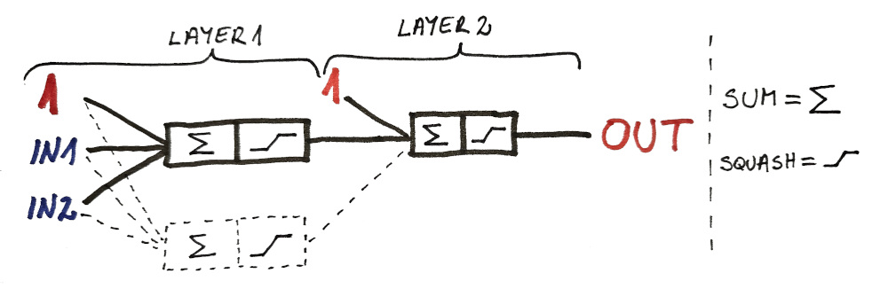
To fix this we need at least 3 neurons in 2 layers, but let’s start step by step…
HUGE learning problem
Single neuron (perceptron) was invented in 1957.
And yes, it didn’t require a genius to arrive at the idea that stacking them into layers would result in more powerful (non-linear) behavior.
However, it took nearly 3 decades (until 1986) before someone came up with an algorithm that could train this neural net (called backpropagation).
Before that, people thought neural nets will never be able to do anything useful (can you imagine that).
MY PROMISE
Since backpropagation includes derivatives (and I promised we’re not going to use derivatives, or any other complex math)… therefore… no derivatives. ✅
Why?
Because there’s a (much) simpler way to train the network.
If it’s so simple why wasn’t it discovered in 1957?
It was, but it couldn’t be used back then.
So what changed?
The difference between now and then is… UNGODLY AMOUNT OF AVAILABLE COMPUTING POWER.
Today, your average laptop is more powerful than all the computers (mainframes) in 1957 (combined).
(probably by a factor of 1 million or some crazy 💩)
Learning algorithm
How are we going to calculate new weights?
We won’t.
Instead, we’re going to guess them.
Think of it as Bitcoin mining, but instead it’s neuron weights Monte Carlo mining.
(and it’s gradual guessing, similar to genetic algorithms)
STEPS
First we initialize the network with random weights (just as we did before).
Then we chose one weight at random and change it slightly.
And then we test the output.
If the overall error is lower than before we keep the new (updated) weights.
If it’s higher, we revert back to previous version.
And that’s it.
The Code
Each neuron has it’s own weights. Since we have 3 neurons in 2 layers, we’re going to name our weight variables accordingly.
// 1st neuron, 1st layer
double[] weights1Layer1 = [0.5, 0.5, 0.5];
// 2nd neuron, 1st layer
double[] weights2Layer1 = [0.5, 0.5, 0.5];
// 1st neuron, 2nd layer
double[] weights1Layer2 = [0.5, 0.5, 0.5];
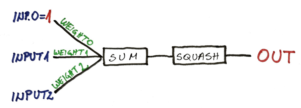
CALCULATING OUTPUT
We calculate this neuron by neuron. We start from the LAYER1 and then the outputs are fed into the third neuron in LAYER2.
double prediction1Layer1 = getPrediction(inputs[i], weights1Layer1);
double prediction2Layer1 = getPrediction(inputs[i], weights2Layer1);
double prediction1Layer2 = getPrediction([prediction1Layer1, prediction2Layer1], weights1Layer2);
The only difference from the previous code is now we have to pass the specific weights (that we wish to use) to the function.
(because now we have more than one)
double getPrediction(double[] inputs, double[] weights) {
	double[] weightedInputs = [1.0] ~ inputs;
	weightedInputs[] *=  weights[];
	double weightedSum = weightedInputs.array.sum;
	double prediction = sigmoid(weightedSum);
	return prediction;
}
RANDOM WEIGHT UPDATE
We don’t do anything wild, we just update existing weight by 0.01 (in either direction)
void updateRandomWeight() {
	double[] selectedWeights = [weights1Layer1,
				    weights2Layer1,
				    weights1Layer2
				    ].choice(rand);
	int index = [0, 1, 2].choice(rand);
	double value = [-0.01, +0.01].choice(rand);
	backupWeights();
	selectedWeights[index] += value;
}
And in case our neurons have different number of weights (which is going to be most of the time) we can use more general solution:
// replace this:
int index = [0, 1, 2].choice(rand);

// with this:
int index = to!int(selectedWeights.length).iota.choice(rand);
Before we change the weights we need to back up / save previous state (in case our change made things worse)…
void backupWeights() {
	backupWeights1 = weights1Layer1.dup;
	backupWeights2 = weights2Layer1.dup;
	backupWeights3 = weights1Layer2.dup;
}
…as well as restore them after we realize predictions got worse:
void restoreWeights() {
	weights1Layer1 = backupWeights1.dup;
	weights2Layer1 = backupWeights2.dup;
	weights1Layer2 = backupWeights3.dup;
}
The rest is pretty much the same as before. Here is the final code:
import std.stdio : pp = writeln;
import std.algorithm : sum, map;
import std.array : array;
import std.math.trigonometry : tanh;
import std.math.algebraic : abs;
import std.random : Random, choice;
import std.conv : to;
import std.range : iota;

auto rand = Random(1);
double[] backupWeights1 = [];
double[] backupWeights2 = [];
double[] backupWeights3 = [];

// 1st neuron, 1st layer
double[] weights1Layer1 = [0.5, 0.5, 0.5];
// 2nd neuron, 1st layer
double[] weights2Layer1 = [0.5, 0.5, 0.5];
// 1st neuron, 2nd layer
double[] weights1Layer2 = [0.5, 0.5, 0.5];

// SIMPLE EXAMPLE

double[][] inputs = [
	[0.0, 0.0], // 1
	[0.0, 1.0], // 0
	[1.0, 0.0], // 0
	[1.0, 1.0], // 1
];
double[] outputs = [1,0,0,1];

// MARKET EXAMPLE

//double[][] inputs = [
//	[0.1, 0.2], // 0
//	[0.5, 1.0], // 0
//	[1.0, 0.5], // 0
//	[1.0, 1.0], // 0
//	[0.0, 0.0], // 0

//	[0.5, 0.5], // 1
//	[0.5, 0.25], // 1
//	[0.25, 0.5], // 1
//	[0.25, 0.75], // 1
//	[0.75, 0.25], // 1
//];
//double[] outputs = [0,0,0,0,0, 1,1,1,1,1];

double sigmoid(double input) { return (tanh(input) + 1) / 2.0; }

double getPrediction(double[] inputs, double[] weights) {
	double[] weightedInputs = [1.0] ~ inputs;
	weightedInputs[] *=  weights[];
	double weightedSum = weightedInputs.array.sum;
	double prediction = sigmoid(weightedSum);
	return prediction;
}

void backupWeights() {
	backupWeights1 = weights1Layer1.dup;
	backupWeights2 = weights2Layer1.dup;
	backupWeights3 = weights1Layer2.dup;
}

void restoreWeights() {
	weights1Layer1 = backupWeights1.dup;
	weights2Layer1 = backupWeights2.dup;
	weights1Layer2 = backupWeights3.dup;
}

void updateRandomWeight() {
	double[] selectedWeights = [weights1Layer1,
				    weights2Layer1,
				    weights1Layer2
				    ].choice(rand);
	int index = to!int(selectedWeights.length).iota.choice(rand);
	double value = [-0.01, +0.01].choice(rand);
	backupWeights();
	selectedWeights[index] += value;
}

void trainNetwork() {
	double maxError = outputs.length;
	for (int n = 0; n < 10000; n++) { // 10.000 times through the data
		double allDataError = 0;
		string printing = "";
		updateRandomWeight();
		for (int i = 0; i < inputs.length; i++) {
			double prediction1Layer1 = getPrediction(inputs[i], weights1Layer1);
			double prediction2Layer1 = getPrediction(inputs[i], weights2Layer1);
			double prediction1Layer2 = getPrediction([prediction1Layer1, prediction2Layer1], weights1Layer2);
			printing ~= to!string(inputs[i]) ~ " : " ~ to!string(prediction1Layer2) ~ " --> " ~to!string(outputs[i]) ~ "\n";
			double error1Layer2 = prediction1Layer2 - outputs[i];
			//allDataError += abs(error1Layer2);
			allDataError += error1Layer2 * error1Layer2;
		}
		if (allDataError < maxError) {
			maxError = allDataError;
			pp(maxError);
			pp(weights1Layer1);
			pp(weights2Layer1);
			pp(weights1Layer2);
			pp(printing);
			pp();
		}
		else {
			restoreWeights();
		}
	}
}

void main() {
	trainNetwork();
	pp("=====");
	pp();
	pp(weights1Layer1);
	pp(weights2Layer1);
	pp(weights1Layer2);
	pp();
}
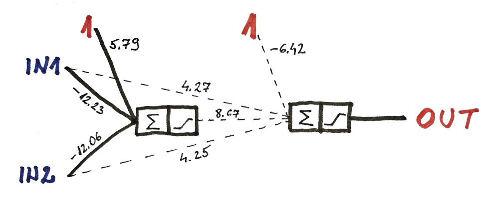
And here are the training results:
// maxError:
// 0.000219457

// weights:
// [-2.41, 4.71, -5.09]
// [2.55, 4.83, -4.86]
// [-2.53, -4.98, 5.04]

// predictions
// [0, 0] : 0.992454 --> 1
// [0, 1] : 0.00695265 --> 0
// [1, 0] : 0.00783815 --> 0
// [1, 1] : 0.992737 --> 1
General guidelines
These are by no means written in stone and depending on the situation you might break them all.
However, these are good as guiding posts before you gain more experience and test a lot of different stuff yourself.
CALCULATING ERRORS
You may have seen this part of code and wondered why do I prefer one over the other:
// absolute error values
allDataError += abs(error1Layer2);

// vs. squared error
allDataError += error1Layer2 * error1Layer2;
First, to clear the obvious, we must use some absolute value of errors. Otherwise, let’s say we had error in one direction (-1) and another error (+1). Then, if we summed those up, we might (falsely) conclude our network didn’t make any errors.
(because the sum of those two errors is zero)
On the other hand, abs() function will (correctly) tell us out total error amount is 2.
However, simple absolute value is not enough because very frequently training can stop progressing before finding optimal solution. Especially if the majority of the predictions are good.
Personally, I use squared error because it prevents situations where network can be massively wrong in any single prediction.
And especially in finance, I’d rather be slightly off frequently instead of one time batshit crazy that wipes out my account.
Besides, even when training XOR, (using the plain abs error values) a lot of times the network gets stuck and doesn’t get trained optimally.
So definitely use squared error.
NUMBER OF ITERATIONS
But how do I know how many iterations to loop through before my network is “completely trained”?
I really don’t in advance.
I start with 100, then move to 1,000 then 10,000… 20k, and so on.
I’m printing out the total error and as long as I see it’s significantly reducing I continue training. But you will see that after some point you get diminishing returns.
This all depends on how much data you have and how much time you want to spend training. (especially in the prototyping phase)
For example, if you remember a couple of years back, all the “impressive” feats of “AI” like Dota 2 bots are a lot less impressive when you realize they were trained on 128.000 CPU cores.
(that is not a typo)
NEURAL NET SIZE
Overall, simpler solutions are usually better than complex solutions. For example, I wouldn’t be surprised if 10-neuron network outperformed 10,000-neuron network.
Because, there is a lot of noise and randomness in financial data.
So having a smaller net makes it impossible to factor in the noise and you end up with much more stable and reliable model.
Creative structures
Remember when I said you need at least 3 neurons in 2 layers in order to properly model XOR logic?
Well that is only true if you want to have 2 clean simple layers.
However, with better structure, you could solve XOR problem using only 2 neurons.
(solution after 15.000 iterations)
But… as you can imagine… using backpropagation is even more complex when the layers are mixed together.
And this is even more of a reason to use our Monte Carlo weight guessing method.
Implementation is equally simple for whatever neural net structure you try it on.
double prediction1Layer1 = getPrediction(inputs[i], weights1Layer1);
double prediction1Layer2 = getPrediction(inputs[i] ~ prediction1Layer1, weights1Layer2);
MORE IDEAS
As you can see, making more intricate neural networks:
- can lead to capturing more complex behavior (XOR)
- without more complex code
As a result, you can quickly experiment with different types of networks without significant changes to the code.
And this is why Monte Carlo weight finding is the best algorithm for training neural nets (in finance). Even though it does use slightly more computer time to train, we are vastly more efficient when coding / prototyping.
NEXT LESSON:
Single Neuron Market Predictions