Limits of The Single Neuron (AI)

(this is part 3 of the “AI for Finance Course“)

In previous lesson, we saw significant improvements when it comes to handling low input values (including zero).

However this is by far the end of the complexity we can find in our data.

In fact, it’s the beginning. Just take a look at these inputs:

double[][] inputs = [
	[0.0, 0.0], // 1
	[0.0, 1.0], // 0
	[1.0, 0.0], // 0
	[1.0, 1.0], // 1
];
double[] outputs = [1,0,0,1];

(you can reuse the code from previous lesson)

And take a look at the predictions from a trained network:

// [0, 0] : 0.156053 --> 1
// [0, 1] : 0.5      --> 0
// [1, 0] : 0.843947 --> 0
// [1, 1] : 0.966939 --> 1

These are very far from the ideal values we trained this network on.

But what happened?

Didn’t we already trained on these exact (or similar) values?

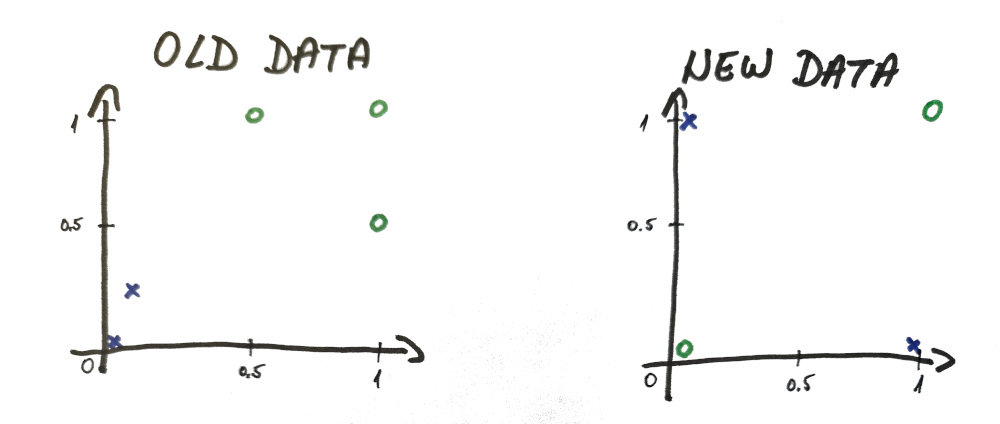
Well almost, but not exactly. Take a look at the data and tell me if you see any difference?

Even though it looks basically the same, there is one BIG difference.

Linearly vs Non-Linearly Separable Data

A single neuron can only make a linear separation between the data. Be it 2-dimensional line (like in our simplified example) or n-dimensional plane, it’s all the same.

And our new data is not linearly separable (i.e. there is no line you can physically draw that will correctly divide these 2 sets of data).

⓵ – horizontal line – top and bottom contain a mixture of both ❌ and 🅾️

⓶ – vertical line – top and bottom contain a mixture of both ❌ and 🅾️

⓷ – this line managed to have only ❌ values on the top and both 🅾️ values at the bottom BUT the second ❌ value also got mixed at the bottom

This is as far as single neuron can go and this is the reason we need to have more neurons.

In our next lesson I’m going to cover how multiple neurons can easily be trained to separate this data.

Market Data Example

To continue with our fictional agricultural company (AgroX)… we said it fairs well when there is plenty of sun and rain.

But we all know from experience that there is such a thing as too much sun and too much rain.

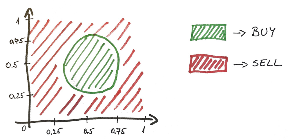
Let’s say, ideally, both values should fall between 0.25 and 0.75 in order for company to have a successful harvest. Otherwise the plants suffer (as well as the company’s profits).

Here is a visual representation of the solution…

And as you can imagine, this problem is not linearly separable.

The Code

I’m including the full code with new inputs so you can test it yourself and try and play with the values.

What you will see is whenever you enter training examples that you cannot separate with a straight line by hand, the neuron (perceptron) cannot do it either.

import std.stdio : pp = writeln;
import std.algorithm : sum;
import std.array : array;
import std.math.trigonometry : tanh;


double[] weights = [0.5, 0.3, 0.4];

// SIMPLE EXAMPLE

double[][] inputs = [
	[0.0, 0.0], // 1
	[0.0, 1.0], // 0
	[1.0, 0.0], // 0
	[1.0, 1.0], // 1
];
double[] outputs = [1,0,0,1];

// MARKET EXAMPLE

//double[][] inputs = [
//	[0.1, 0.2], // 0
//	[0.5, 1.0], // 0
//	[1.0, 0.5], // 0
//	[1.0, 1.0], // 0
//	[0.0, 0.0], // 0

//	[0.5, 0.5], // 1
//	[0.5, 0.25], // 1
//	[0.25, 0.5], // 1
//	[0.25, 0.75], // 1
//	[0.75, 0.25], // 1
//];
//double[] outputs = [0,0,0,0,0, 1,1,1,1,1];

double sigmoid(double input) { return (tanh(input) + 1) / 2.0; }

void updateWeights(double prediction, double[] inputs, double output) {
	double error = prediction - output;
	pp("error: ", error);
	double[3] errorCorrections = ([1.0] ~ inputs)[] * error;
	weights[] -= errorCorrections[];
	pp("weights: ", weights);
}

double getPrediction(double[] inputs) {
	double[3] weightedInputs = ([1.0] ~ inputs)[] * weights[];
	double weightedSum = weightedInputs.array.sum;
	double prediction = sigmoid(weightedSum);
	return prediction;
}

void trainNetwork() {
	for (int n = 0; n < 1000; n++) { // 1000 times through the data
		for (int i = 0; i < inputs.length; i++) {
			double prediction = getPrediction(inputs[i]);
			updateWeights(prediction, inputs[i], outputs[i]);
		}
	}
}

void main() {
	pp("weights: ", weights);
	trainNetwork();

	// TESTING
	pp();
	pp(inputs[0], " : ", getPrediction(inputs[0]));
	pp(inputs[1], " : ", getPrediction(inputs[1]));
	pp(inputs[2], " : ", getPrediction(inputs[2]));
	pp(inputs[3], " : ", getPrediction(inputs[3]));
	//pp(inputs[4], " : ", getPrediction(inputs[4]));
	//pp(inputs[5], " : ", getPrediction(inputs[5]));
	//pp(inputs[6], " : ", getPrediction(inputs[6]));
	//pp(inputs[7], " : ", getPrediction(inputs[7]));
	//pp(inputs[8], " : ", getPrediction(inputs[8]));
	//pp(inputs[9], " : ", getPrediction(inputs[9]));
	pp();
}

Here are the prediction results for our simple dataset example (from the beginning of this lesson)…

// [0, 0] : 0.156053 --> 1
// [0, 1] : 0.5      --> 0
// [1, 0] : 0.843947 --> 0
// [1, 1] : 0.966939 --> 1

…as well as the prediction results for the market data. As you can see, it’s not even close. But we will fix this in our next lesson.

// [0.1, 0.2] : 0.892013   : 0
// [0.5, 1] : 0.916822     : 0
// [1, 0.5] : 0.986684     : 0
// [1, 1] : 0.977913       : 0
// [0, 0] : 0.884867       : 0

// [0.5, 0.5] : 0.948577   : 1
// [0.5, 0.25] : 0.959781  : 1
// [0.25, 0.5] : 0.902     : 1
// [0.25, 0.75] : 0.876768 : 1
// [0.75, 0.25] : 0.97952  : 1

NEXT LESSON:
Multi-Neuron Network Explained (AI)