(this is part 2 of the “AI for Finance Course“)
Previously, you might have seen how the most basic form of a neuron simply cannot handle all the data that is thrown at it, specifically low values.
This means, if both of our inputs are zero, regardless of how good our weights are tuned, the sum will always be zero.
(and consequently, sigmoid function will always be 0.5)
// [0.1, 0.2] : 0.612728 <-- problem
// [0.5, 1] : 0.908376
// [1, 0.5] : 0.999506
// [1, 1] : 0.998647
// [0, 0] : 0.5          <-- problem
This was clearly visible from our predictions after our neuron (perceptron) was fully trained:
- no matter what I do
- or how long I train it
- or how many trillions of data points I provide
=> the output for [0, 0] inputs will always be 0.5
Fixing Near-Zero Inputs
The solution is very simple. We just need to add the “constant” term to allow our neuron (which is basically just a function) to have non-zero outputs for purely-zero inputs.
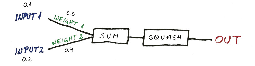
So instead of having a neuron like this…
…we’re going to have a neuron like this:
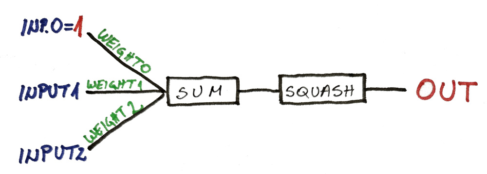
INPUT0 is always going to be 1, and it will never change. The only thing that can be changed is WEIGHT0.
Now, in our previous example without a constant INPUT0, we can see that our output was always 0.5 when all our inputs were zero.
// [0.1, 0.2] : 0.612728 <-- problem
// [0.5, 1] : 0.908376
// [1, 0.5] : 0.999506
// [1, 1] : 0.998647
// [0, 0] : 0.5          <-- problem
In this case if we set our WEIGHT0 to -100 (or whatever big negative number), our squashing function will be close to zero.

And in our hypothetical AgroX example, this would mean we should sell this stock.
Reminder:
- INPUT1 = 0 means the temperature was lowest on record
- INPUT2 = 0 means the rain was lowest on record
This means the crop season will be terrible, therefore sales will be low, and stock price will fall. So we should sell (i.e. out network should output zero)
Fixing The Code
There is almost no change to the code from the previous lesson, so I’m not going to analyze it a bit by bit. There are only 3 lines changed as indicated by the comments in the code.
The only difference is:
- now there’s going to be 3 weights instead of one
- and I’ll add a constant term 1.0 to the inputs
Everything else will stay the same. I will re-run the training and we will see if the outputs are now fixed.
(i.e. whether the error is lower)
Here is the code in its entirety:
import std.stdio : pp = writeln;
import std.algorithm : sum;
import std.array : array;
import std.math.trigonometry : tanh;


double[] weights = [0.5, 0.3, 0.4]; // changed line

double[][] inputs = [
	[0.1, 0.2], // 0 - bad year - sell
	[0.5, 1.0], // 1 - avg temp & best rain - buy
	[1.0, 0.5], // 1 - best temp & avg rain - buy
	[1.0, 1.0], // 1 - best temp & best rain - BUY
	[0.0, 0.0], // 0 - worst year on record - SELL!!!
];

double[] outputs = [0, 1, 1, 1, 0];

double sigmoid(double input) { return (tanh(input) + 1) / 2.0; }

void updateWeights(double prediction, double[] inputs, double output) {
	double error = prediction - output;
	pp("error: ", error);
	double[3] errorCorrections = ([1.0] ~ inputs)[] * error; // changed
	weights[] -= errorCorrections[];
	pp("weights: ", weights);
}

double getPrediction(double[] inputs) {
	double[3] weightedInputs = ([1.0] ~ inputs)[] * weights[]; // changed
	double weightedSum = weightedInputs.array.sum;
	double prediction = sigmoid(weightedSum);
	return prediction;
}

void trainNetwork() {
	for (int n = 0; n < 1000; n++) { // 1000 times through the data
		for (int i = 0; i < inputs.length; i++) {
			double prediction = getPrediction(inputs[i]);
			updateWeights(prediction, inputs[i], outputs[i]);
		}
	}
}

void main() {
	pp("weights: ", weights);
	trainNetwork();

	// TESTING
	pp();
	pp(inputs[0], " : ", getPrediction(inputs[0]));
	pp(inputs[1], " : ", getPrediction(inputs[1]));
	pp(inputs[2], " : ", getPrediction(inputs[2]));
	pp(inputs[3], " : ", getPrediction(inputs[3]));
	pp(inputs[4], " : ", getPrediction(inputs[4]));
	pp();
}
And if you take a look at the outputs now, they are nearly perfect:
// [0.1, 0.2] : 0.00214298
// [0.5, 1] : 0.999116
// [1, 0.5] : 0.999389
// [1, 1] : 0.999997
// [0, 0] : 7.97197e-05 <-- excellent
And just as a reminder, these were our previous predictions where our neuron (perceptron) didn’t have the “constant” term.
(also known as bias)
// [0.1, 0.2] : 0.612728 <-- problem
// [0.5, 1] : 0.908376
// [1, 0.5] : 0.999506
// [1, 1] : 0.998647
// [0, 0] : 0.5          <-- problem
Also it might be interesting to see how the weights changed:
// OLD WEIGHTS
// [4.31008, -1.00806]

// NEW WEIGHTS
// [-4.71846, 5.73579, 5.36586]
In the end, WEIGHT0 wasn’t -100 in but it was large enough for our function to output near-zero value of 7.97197e-05
Now that we have the best possible neuron we can have, let’s jump into the next lesson:
NEXT LESSON:
Limits of The Single Neuron (AI)